USING R LANGUAGE BSTS PACKAGE FOR MODELLING BAYESIAN STRUCTURAL TIME SERIES

BSTS model

In Bayesian structural models, the time series is represented as a sum of unobservable components, which can be interpreted, for example, as trend, seasonality, cycle, error. The Bayesian approach to statistical problems is fundamentally probabilistic. A joint probability distribution is used to describe the relationships between all the unknowns and the data. The inference is then based on a conditional probability distribution of the unknowns given the observed data — an a posteriori distribution. Using the internal consistency of the probability system, the posterior distribution extracts relevant information from the data and provides a complete and consistent representation of all state variables (including unobserved components) to discover causal relationships between the prediction and observed data. The use of the posterior distribution to solve specific inference and decision-making problems is in this case quite straightforward. Thus, compared to other models, the BSTS model allows us to account for uncertainty in the data and complex relationships between observed variables.

The fitting of structural time series models is done using the Kalman filter and the Markov chain Monte Carlo method (MCMC). To estimate and simultaneously regularize the regression coefficients, the so-called spike-and-slab regression, a type of Bayesian linear regression in which a particular hierarchical a priori distribution for the regression coefficients is chosen so that only a subset of possible regressors is retained. Some regression coefficients are assigned a high a priori probability that they are zero. Subsequently, MCMC sampling of the coefficients from the resulting posterior distributions reveals many coefficients to be exactly zero. This regularization mechanism allows us to efficiently select the most important predictors and in parallel to get rid of multicollinearity, so that a large number of predictors can be included in Bayesian structural models without the risk of overtraining.

Software experiments

The applicability of the BSTS model to estimate the parameters of the temperature time series was investigated in software experiments. In the experiment, we used temperature data in Tomsk for the last 5 years, received from the All-Russian Research Institute for Hydrometeorological Information — World Data Center (RIHMI-WDC) [9]. That is, the object of the study was a time series composed of average daily air temperatures in Tomsk for the period from 2017 to 2022 (Fig. 1). The statistical modeling language R and bsts package were used as tools [10].

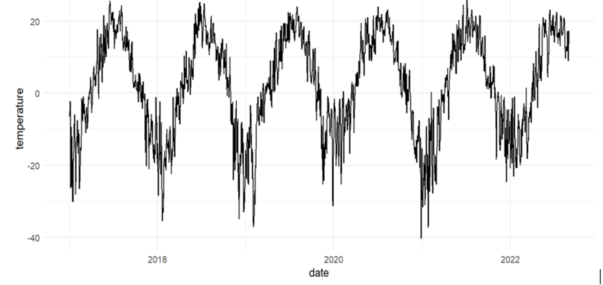
Figure 1. Average daily air temperatures in Tomsk

First, import the data and present it as a time series.

Next, we decompose the time series to understand its structure.

Figure 2 shows the result of decomposition of this series. The figure shows that this series has an obvious annual seasonality, but no significant trend.

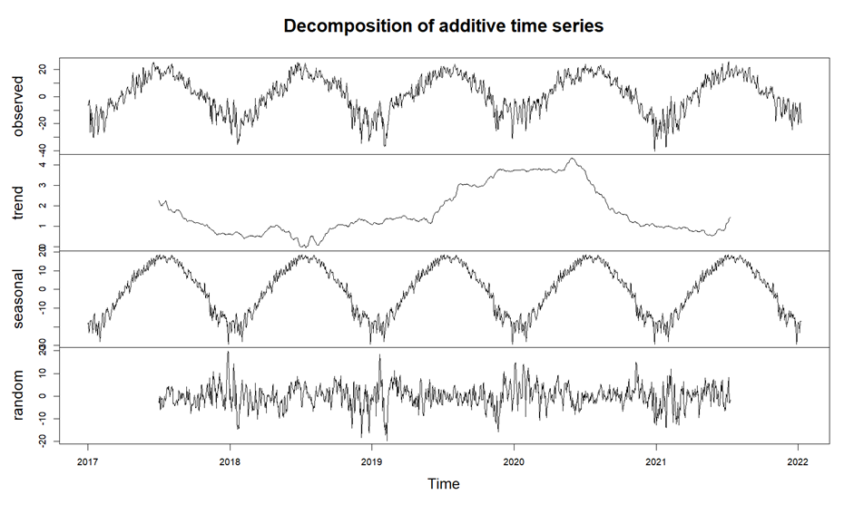
Figure 2. The result of time series decomposition

Then we split the data into a training sample and a validation sample (Fig. 3). The forecast period is set to 200 days.

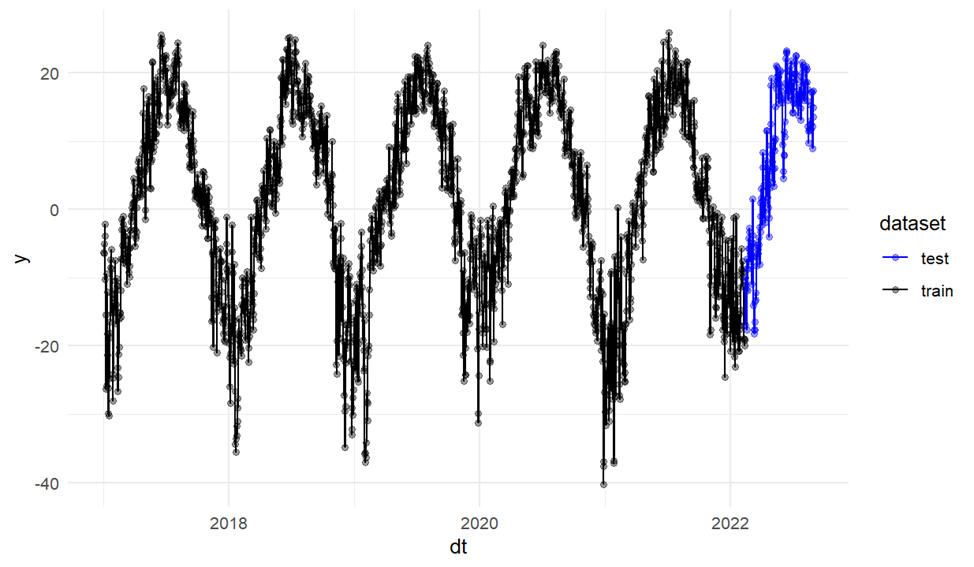
Figure 3. Training and test samples

Next comes the fitting of the model.

Figure 4 shows the result of the model fitting.

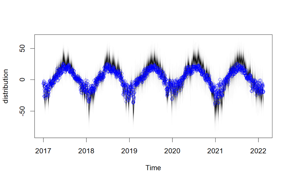
Figure 4. Result of model fitting

Next are the forecast and the visual assessment of the forecast. Figure 5 shows the result of the forecast. Blue represents the forecast. In yellow are the data from the validation sample.

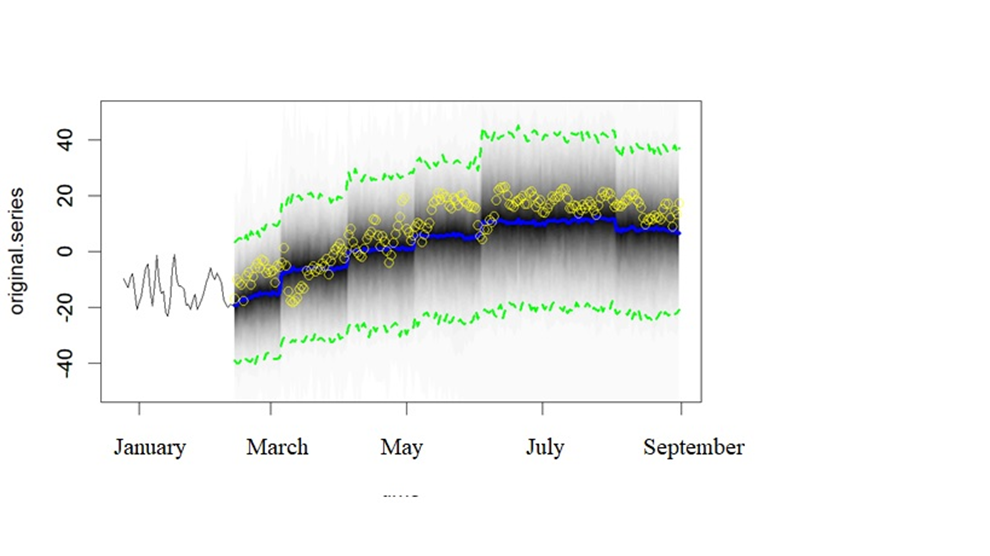
Figure 5. Forecast result

Next, we calculate the mean absolute specific error (MAPE).

Figure 6 shows the resulting error value.

Figure 6. Mean absolute specific error

Conclusion

A software experiment scheme was developed to build and study a Bayesian structural time series model (BSTS-model). The data was sampled from long-term observations of surface atmospheric temperature in Tomsk. The statistical modeling language R and the package bsts (Bayesian Structural Time Series), a package for computing time series regression using dynamic linear models and a Monte Carlo fit based on the Markov chain method (MCMC), were used as the toolbox. Bayesian inference is a very efficient method for time series analysis, but there are many features in the BSTS model that have yet to be explored.

References:

1. Bayesian structural time series // wiki5.ru. URL: https://wiki5.ru/wiki/Bayesian_structural_time_series (accessed 14.04.2023).